Fluid Simulation for Computer Graphics Reading Note

It is an reading note of “Fluid Simulation for Computer Graphics”, related about fluid simulation coding, such as SPH, Level Set, PIC/FLIP and so on.

The article can’t cover all details, it just a reading note. Implementation details are so complex that it is recommended to have a look on original source.

Also see:

http://rlguy.com/gridfluidsim/

Chapter 1: The Equations of Fluids

Force

What is the pressure? Whatever it takes to keep the fluid at constant volume.

It measures the imbalance in pressure at the position of the particle is simply to take the negative gradient of pressure

Viscosity force tries to resist deforming. It tries to make our particle move at the average velocity of the nearby particle.

The differential operator that measures how far a quantity is from the average around it is Laplacian operator , so viscosity force is

Incompressibility

Incompressibility means volume doesn’t change. It is . How to get NS eq ?

The integration should be true for any choice of , any region of fluid. The only continuous function that integrates to zero independent of the region of integration is zero itself. Thus the integrand has to be zero everywhere.

One of the tricky parts of simulating incompressible fluids is making sure that the velocity field stays divergence-free. This is where the pressure comes in.

Optimization View: think of the incompressibility condition as a constraint and the pressure field as the Lagrange multiplier.

Dropping Viscosity

Most numerical methods for simulating fluids unavoidably introduce errors that can be physically reinterpreted as viscosity, so even if we drop viscosity in the equations, we will still get something that looks like it.

Boundary Conditions

Wall condition

…

Free surface

Fluid area and air area can’t share same update process, because air is 700 times lighter than water, it’s not able to have that big of an effect on the water anyhow.

Bubbles are another topic.

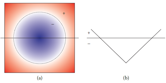
So instead we make the modeling simplification that the air can be represented as a region with constant atmospheric pressure. In actual fact, since only differences in pressure matter (in incompressible flow), we can set the air pressure to be any arbitrary constant: zero is the most convenient. Thus a free surface is one where p = 0, and we don’t control the velocity in any particular way.

The other case in which free surfaces arise is where we are trying to simulate a bit of fluid that is part of a much larger domain. We obviously can’t afford to simulate the entire atmosphere of the Earth, so we will just make a grid that covers the region we expect to be "interesting.

For smaller-scale liquids, surface tension can be very important. So curvature of free surfaces is important.

Bubbles

For normal water, we consider volume and momentum. For bubbles, we only condsider volume. Because air is much lighter than water, and so usually might not be able to transfer much momentum to water.

But bubbles may immediately collapse (there’s no pressure inside to stop them losing their volume). To handle this kind of situation, you need either hacks based on adding bubble particles to a free surface flow, or more generally a simulation of both air and water (called two-phase flow, because there are two phases or types of fluid involved).

Chapter 2: Overview of Numerical Simulation

Splitting

Split into:

Use Taylor series to prove firse-order-accurate.

Simpler equation has simpler method.

We have better method .

may be in parallel or not.

Splitting the Fluid Equations

In advection part, quantity is anything, not just velocity .

For body force part, forward euler is fine.

Pressure part is to make sure . Here we will project velocity and enforce the solid wall boundary conditions.

Advection should only be done in a divergence-free velocity field. So sequence matters.

1. advect

2. add body force

3. project

Time Steps

Find a minimal time step that suits all steps: advect, add body force, project.

If frame interval > simulation delta time , then run simulation multiple times, until total simulation time >= .

MAC Grid

Problem of central difference

First-order central difference:

First-order forward or backward difference:

First-order central difference has a major problem in that the derivative estimate at grid point i completely ignores the value qi sampled there.

Why ignoring qi is terrible: jagged function has more probability to be estimate as constant function. For example, to produce using first-order central difference, but not using first-order forward or backward difference.

I think it is similar with Undersampling. Nyquist-Shannon sample Theorem says that for an accurate representation of the baseband signal, the sample rate must be at least twice the highest frequency component. Aliasing happens when the sampling rate falls below this limit (the Nyquist Rate).

Here you can analogize aliasing to becoming close to 0.

Fig: Undersampling

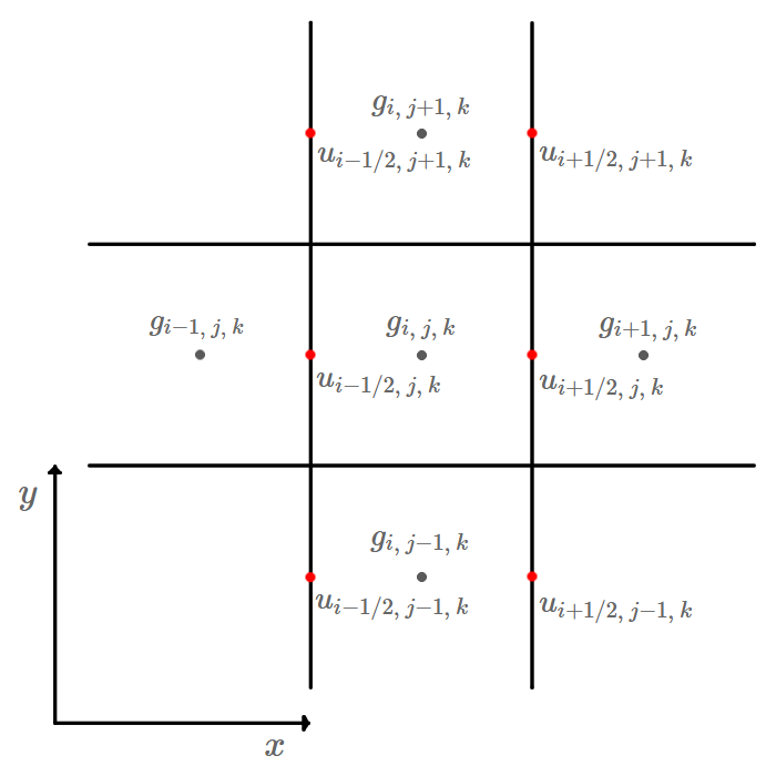
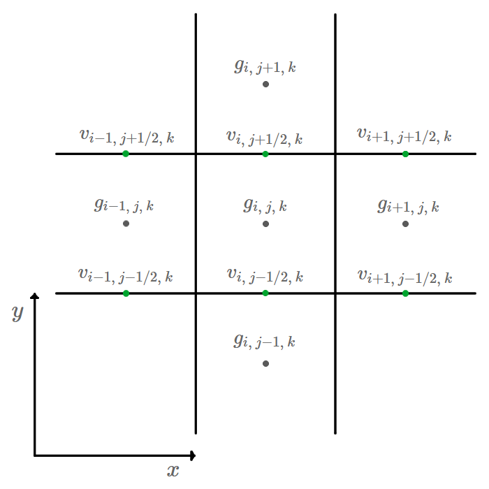
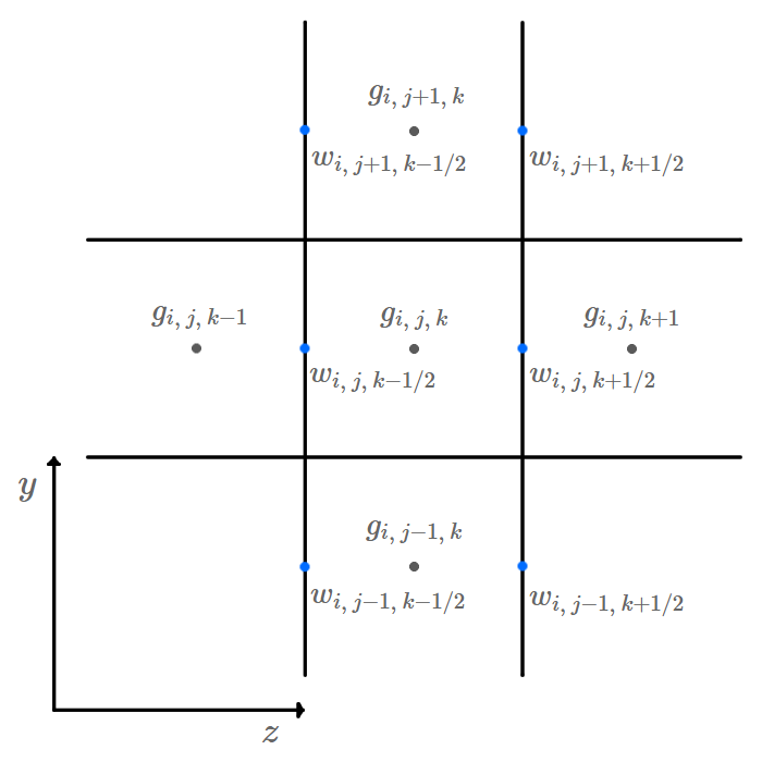
MAC Velocity Grid

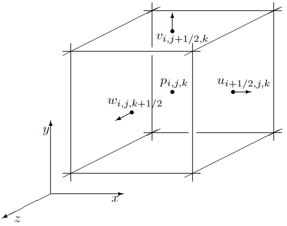
MAC Grid is a staggered grid designed to solve incompressibility.

Why to use MAC Grid: we can use accurate central differences for the pressure gradient and for the divergence of the velocity field without the usual disadvantages of central differences

Pressure is defined at center of cell.

is defined at center of X plane of cell.

is defined at center of Y plane of cell.

is defined at center of Z plane of cell.

Fig: MAC Grid Veocity u

Fig: MAC Grid Veocity v

Fig: MAC Grid Veocity w

Fig: One cell from the three-dimensional MAC grid

If pressure grid has dimensions , then grid has dimensions , grid has dimensions , grid has dimensions .

The half-index notation works well for describing velocity components in this document, but does not translate well into a programming implementation where arrays use integer indexing. The following table demonstrates how half-index notation will be translated into classic array integer indexing:

Half Index	Integer Index

Using staggered grid, we can get unbiased second-order accuracy of a central difference:

The staggered MAC grid is perfectly suited for handling pressure and incompressibility, but it’s frankly a pain for other uses. For example, if we actually want to evaluate the full velocity vector somewhere, we will always need to use some kind of interpolation even if we’re looking at a grid point.

For an arbitrary location:

Dynamic Sparse Grids

Problem:

1. If fluid region change over time, using a static grid that covers the entire region can be wasteful

   Solution: Adjust the grid dimensions and where it lies in space at every time step

   • For fluid: water surface with padding

   • For smoke: smoke can extends into whole space. So calc SDF according smoke concentration.

2. Memory access efficiency on modren hardware

   Assume that grid is row-major layout, and row order is . Distance between and will be

   So we can expect more page faults and cache misses.

3. Fluid occupies only a small fraction of the volume of its bounding box

   For example: river, waterfall, pouring water…

Using hash table to map index to a large virtual grid (such as along each dimension by signed 32-bit integers in each coordinate). The grid is large enough so you don’t need to move grid origin.

Since we only store the blocks of the grid we care about, this is a sparse structure and we don’t waste storage or processing on voxels far from the action…

Because we map blocks of voxels rather than individual voxels, the overhead of the associative data structure can be minimized; meanwhile operations inside a block have extremely good data locality.

Code 2D before 3D

Bug about copying and pasting

Chapter 3: Advection Algorithms

Advection should only be called with a divergence-free velocity field

Semi-Lagrangian Advection

Forward Euler

Forward Euler is unconditionally unstable.

About stability region of forward Euler. The eigenvalues of the Jacobian generated by the central difference are pure imaginary, thus always outside the region of stability.

Problem of spatial discretization

Difference seems like pretty accurate estimate of the derivative, but it has dispersion problem.

High-frequency jagged components of quantity, like , erroneously register as having zero or near-zero spatial derivative, and so don’t get evolved forward in time or at least move much more slowly than the velocity u they should move at.

Meanwhile the low frequency components are handled accurately and move at almost exactly the right speed u. Thus the low frequency components end up separating out from the high-frequency components, and you are left with all sorts of strange high-frequency wiggles and oscillations appearing and persisting that shouldn’t be there!

I have known two kinds of problem in discretization: dissipation and dispersion, but I think the view of frequency is novel. When I learnt compute fluid, I had no concept about it.

Semi-Lagrangian Advection

…

I have learnt it when reading Stable Fluid.

If you are using MAC Grid, then your advence velocity should be interpolated from MAC Grid.

Boundary Conditions

When backtrace the start point of particle, it may locate outside of boundary.

Two reasons:

1. The start point is in inlet

2. The start point shouldn’t be outside, it is about numerical error about forward Euler or Runge-Kutta step when calculate the position of start point

The first reason is artificially designed, we have known inlet condition to solve it.

For the second reason, the appropriate strategy is to extrapolate the quantity from the nearest point on the boundary. So the start point outside can use the extrapolated quantity.

If the quantity outside is known, then extrapolation will be easy.

If the quantity outside is unknown, there is two ways:

1. Extrapolation

2. For fluid:

   Find nearest point in fluid surface, which means minimize the distance from surface to start point, then interpolate quantity at the nearest point found.

   For solid wall:

   Normal velocity condition, or for viscous flow, take the shortcut of just using the solid’s velocity.

Time Step Size

Semi-Lagrangian Advection is unconditionally stable, becuase new value is copied from old value, so new value will never be larger than old value.

To avoid artifacts, time step still has limit? I haven’t try it.

CFL condition

From view of domain of dependence, the numerical domain of dependence, at least in the limit, must contain the true domain of dependence if we want to get the correct answer.

CFL condition depicts how small your is can you say close to limit.

CFL condition: to make result accurate

stability condition: to make update stable

CFL number: a parameter in CFL condition

CFL number represents the maximum number of grid cells the information can propagate

If a method unconditionally unstable but fit CFL condition, it will still covergence to accurate result.

Diffusion

Assume that we have find start point of particle, then we should know the quantity at start point, so we use interpolation. It introduces diffusion, or in signal-processing terminology, we have a low-pass filter.

Prove the Semi-Lagrangian Advection introduce dissipation

…

Reducing Numerical Diffusion

As we saw in the last section, the problem mainly lies with the excessive averaging induced by linear interpolation (of the quantity being
; linearly interpolating the velocity field in which we trace is not the main culprit and can be used as is).

Solution: use sharper interpolation

Cubic Interpolation:

Where means fraction between grid points and . So means , means , means , means .

It can be derived from Lagrange Interpolation, base point are , , , .

This algorithm also has another form. Derived from another way Paul Bourke’s Cubic Interpolation Page

Where is same as below.

In two or three dimensions, you can cubic interpolation sequentially.

Code example for 3D:

double cubicInterpolate(double p[4], double x) {
    return p[1] + 0.5 * x*(p[2] - p[0] + 
                           x*(2.0*p[0] - 5.0*p[1] + 4.0*p[2] - p[3] + 
                              x*(3.0*(p[1] - p[2]) + p[3] - p[0])));
}

double bicubicInterpolate(double p[4][4], double x, double y) {
    double arr[4];
    arr[0] = cubicInterpolate(p[0], x);
    arr[1] = cubicInterpolate(p[1], x);
    arr[2] = cubicInterpolate(p[2], x);
    arr[3] = cubicInterpolate(p[3], x);
    return cubicInterpolate(arr, y);
}

double tricubicInterpolate(double p[4][4][4], double x, double y, double z) {
    double arr[4];
    arr[0] = bicubicInterpolate(p[0], x, y);
    arr[1] = bicubicInterpolate(p[1], x, y);
    arr[2] = bicubicInterpolate(p[2], x, y);
    arr[3] = bicubicInterpolate(p[3], x, y);
    return cubicInterpolate(arr, z);
}

The weighting coefficients may be negative.

Chapter 4: Level Set Geometry

1. when is a point inside a solid? (the point may be where we traced back to during semi-Lagrangian)

2. what is the closest point on the surface of some geometry?

3. how do we extrapolate values from one region into another?

SDF

Fig: SDF Field. Taken from "Fluid Engine Development"

.

• outside the geometry, is the unit-length vector pointing towards the closest point on the surface

• inside the geometry, is the unit-length vector pointing towards the closest point on the surface

• and on the surface, is the unit-length outward-pointing normal.

This means is the closest point on the surface for any point .

SDF can also be defined as at boundary.

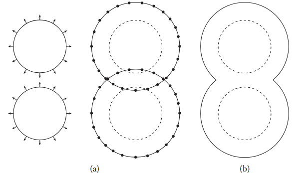
SDF can handle topological change easily. To merge two surface, just get minimum value of two SDF.

Fig: SDF Topology. Taken from "Fluid Engine Development"

Reinitializing SDF

After advection, the SDF field can not keep its distance property. So we should recover it. Luckily, only the SDF value on the surface is correct. So the reinitializeing can start from surface.

Fig: SDF Reinitializing. Taken from "Fluid Engine Development"

Here we prove why the value on the surface is correct.

We can use the advection equation (Equation 3.23) with extra source term to model this propagation problem.

is pseudo-time, because it is not physics simulation but more like a geometric postprocessing.

If source term in right hand side is 0, it means is only carried by the vector field . If a constant is assigned, it means is added to when it travels one distance unit along .

Thus, setting the right-hand side to 1 means we will assign the traveled distance to .

We have discuss the gredient of before, we know that if we assign as distance, then the gredient is 1, it means when travels one distance unit in space along the steepest direction, the value of increase 1.

So if we assign gredient of as direction of reinitializing velocity, then the advection equation will fit its physical meaning.

In other word, substitute

into advection equation, get

which can be further simplified to

Reinitialize outward from the surface, the direction is the same as the gradient, .

On the contrary, reinitialize inward from the surface, we have . Similarly, we have

In summary, reinitializing equation is

Medial Axis

SDF is smooth everywhere except on the medial axis

The medial axis is exactly where there isn’t a unique closest point, such as the center of a sphere and the middle plane inside a flat slab.

Discussion about the gradient breaks down on the medial axis, because the function isn’t differentiable there.

Discretizing Signed Distance Functions

Level set method: signed distance function that has been sampled on a grid

How to get at any point? There are two ways:

1. Interpolate nearby the given point, then differentiate the interpolant of

2. Differentiate at the grid point nearby the given point, then interpolate between which lie in grid.

Usually use thel later way, because if interpolate first, interpolant of may have discontinuities in their derivative between grid cells.

Computing Signed Distance

1. from geom etry (finding closest points and measuring the distance to them).

   geometry is explicitly known

2. from PDEs (solving the Eikonal equation ).

   geometry isn’t explicitly known

Distance to Points

This is algorithm 4 in:

Y.-H. R. Tsai. Rapid and accurate computation of the distance function using grids. J. Comput. Phys., 178(1):175–195, 2002

for i in range(nx):
    for j in range(ny):
        for k in range(nz):
            phi[i][j][k] = infty  # A 3D array of distances
            t[i][j][k] = -1  # A 3D array of integer indices for the closest point

# Initialize the arrays near the input geometry
for e in range(len(all_input_points)):
    pe = all_input_points[e]
    (i,j,k) = get_grid_index_from_position(pe)

    d = length(vec3(i,j,k) - pe)
    if d < phi[i][j][k]:
        phi[i][j][k] = d
        t[i][j][k] = e

# Propagate closest point and distance estimates to the rest of the grid
loop (i,j,k) in a chosen order:
    foreach neighboring grid point (i2,j2,k2) worth considering:
        e = t[i2][j2][k2]

        if e != -1:
            pe = all_input_points[e]

            d = length(vec3(i,j,k) - pe)
            if d < phi[i][j][k]:
                phi[i][j][k] = d
                t[i][j][k] = e

In the first stage we compute exact distance and closest point information directly in the grid cells that surrounding the input points.

The second stage can efficiently propagate information from neighbor to neighbor through the grid.

Both stages don’t need extra data structures.

Loop Order

Two kinds of loop order when propagating information

1. fast marching method

2. fast sweeping method

Fast Marching Method

Grid points should get information about the distance to the geometry from points that are closer, not the other way around

So loop over the grid points going from the closest to the furthest

Facilitated by storing unknown grid points in a priority queue (typically implemented as a heap) keyed by the current estimate of their distance.

Each update, remove the minimum

O(nlogn)

Fast Sweeping Method

For any grid point, in the end its closest point information is going to come to it from one particular direction in the grid—e.g., from (i + 1, j, k), or maybe from (i, j − 1, k), and so on. To ensure that the information can propagate in the right direction, we thus sweep through the grid points in all possible loop orders: i ascending or descending, j ascending or descending, k ascending or descending.

8 combinations in 3D.

For more accuracy, we can repeat the sweeps again; in practice two times through the sweep gives excellent results

O(n), no extra data structures

When using sparse tiled grids

In this case, a hybrid approach is possible. We can run fast sweeping efficiently inside a tile to update distances based on information in the tile and its neighbors, but we can choose the order in which to solve tiles (and re-solve them when neighbors are updated) in a fast marching style. Begin with the tiles containing input points as the set to “redistance”. Whenever a tile has been redistanced with fast sweeping, check to see if the distance value in any face neighbor is more than ∆x larger than the distance stored in this tile: if so, add the neighboring tile to the set needing redistancing.

I can’t understand it.

Finding Signed Distance for a Triangle Mesh

for i in range(nx):
    for j in range(ny):
        for k in range(nz):
            phi[i][j][k] = infty  # A 3D array of distances
            t[i][j][k] = -1  # A 3D array of integer indices for the closest point
            c[i][j][k] = 0  # A 3D array of integers to keep intersection counts along grid edges

# Initialize the arrays near the input geometry
for e in range(len(all_input_triangles)):
    Te = all_input_triangles[e]
    loop grid edges (i,j,k)-(i+1,j,k) which exactly intersect triangle Te  # consistently breaking ties at endpoints
        c[i][j][k]++

        d = distance_to_triangle(vec3(i,j,k), Te)
        if d < phi[i][j][k]:
            phi[i][j][k] = d
            t[i][j][k] = e

# Propagate closest triangle and distance estimates to the rest of the grid
loop (i,j,k) in a chosen order:
    foreach neighboring grid point (i2,j2,k2) worth considering:
        e = t[i2][j2][k2]
        if e != -1:
            Te = all_input_triangles[e]

            d = distance_to_triangle(vec3(i,j,k), Te)
            if d < phi[i][j][k]:
                phi[i][j][k] = d
                t[i][j][k] = e

# Determine signs for inside/outside
foreach horizontal grid line (j,k):
    C = 0
    for i in range(nx):
        if C % 2 == 1:
            phi[i][j][k] = -phi[i][j][k]
        C += c[i][j][k]

Fast sweeping, fast marching, or a hybrid tiled combination can also be used.

Computing the distance between a point and a triangle

Mark W. Jones. 3d distance from a point to a triangle. Technical report, Department of Computer Science, University of Wales, 1995

Assume we are computing the distance between point pe and triangle Te. Firstly, we should find closest point for pe in the triangle,

…

Chapter 5: Making Fluids Incompressible

Project

To solve , use forward euler:

The solving result should met divergence-free condition:

These two equations should be combined to solve pressure, we will see how to discrete them next, and how to substitute one into another.

For the first equation:

For the second equation:

Assume , substitute the :

This equation can be written in matrix form as . It is easy to know that A is a sparse matrix.

This system of linear algebraic equations can be solved using direct or iterative methods.

Considering that the fluid domain can be large and the direct method computationally expensive, using an iterative method may be a better option. Commonly, efficient iterative methods such as conjugate gradient method is used, and acceleration algorithms include preconditioner method and regional equilibrium decomposition algorithm is also used.

When actually constructing Poisson’s equation, boundary conditions also need to be taken into consideration.

It is my understanding when I read the book firstly.

After I read other’s, I found that forward Euler is to find fucture state n+1 with current state n, and backward Euler is to update current state n with known fucture state n+1.

So that is why each elements in forward Euler can be calcuated parallelly, but each elements in backward Euler are coupled. In forward Euler, if you want to predict a point, you only need to fetch its neighbor points’ old value. These old value are read-only. But in backward Euler, to update a point, the neighbor you fetch is also required to be writed when updating other points.

Elements are coupled means that you should solve a problem.

As for pressure solving, The forward-style method would take the current density error to compute pressure. So, in backward sense, we would deduce the pressure by saying that this still-unknown pressure will make the density error to zero. The zero density error means that the density should remain constant, and that leads to

So it is natural to substitute into .

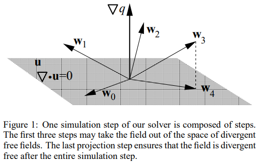
Why is it called projection?

According to Helmholtz-Hodge Decomposition, states that any vector field can uniquely be decomposed into a divergence-free vector field adding with a gredient of a scalar field.

Where .

Poisson equation can be derived from this equation by multiplying both sides by “”.

So now we can say the Poisson eq is equivalent to Helmholtz-Hodge Decomposition, while the Helmholtz-Hodge Decomposition can be written as projection:

Where satisfies , .

So you can see, solving Poisson eq is projecting velocity field to pressure field.

Fig: Velocity Projection. Taken from "Stable Fluid"

Method without projection

If you don’t project velocity field to pressure filed, only solve the divergence-free condition, there is simpler algorithm.

Take 2D as an example,

we need to accomplish .

It can be shorten as:

A quick way is calculating the difference, and distribute it onto the four velocity.

d = u[i+1][j] - u[i][j] + v[i][j+1] - v[i][j]

u[i][j] += d/4
u[i+1][j] -= d/4
v[i][j] += d/4
v[i][j+1] -= d/4

Wall Condition

Considering the wall condition. Wall cell doesn’t have velocity, but if using MAC grid, velocity is defined in cell faces.

So the border between wall and fluid has velocity.

Essentially, distributing d is distributing additional flux of the cell to cell face, to make the cell 0 flux.

But there isn’t flux from wall or to wall, so things change:

Boolean flag

Set represent fluid, represent wall.

d = u[i+1][j] - u[i][j] + v[i][j+1] - v[i][j]
s = s[i+1][j] + s[i-1][j] + s[i][j+1] + s[i][j-1]

u[i][j] += d * s[i-1][j] / s
u[i+1][j] -= d * s[i+1][j] / s
v[i][j] += d * s[i][j-1] / s
v[i][j+1] -= d * s[i][j+1] / s

Here we may access cells out of boundary. A solution is adding border cells.

The current four velocity values being processed, have overlapping value with previous four velocity values. It means that right after you make current four velocity values divergence-free, the previous may get divergence again.

So you should repeat it over and over again, until the whole field coverge.

while velocity field doesn't converge:
    d = u[i+1][j] - u[i][j] + v[i][j+1] - v[i][j]
    s = s[i+1][j] + s[i-1][j] + s[i][j+1] + s[i][j-1]

    u[i][j] += d * s[i-1][j] / s
    u[i+1][j] -= d * s[i+1][j] / s
    v[i][j] += d * s[i][j-1] / s
    v[i][j+1] -= d * s[i][j+1] / s

Copying value

Set for border cells is one method, another method is copying neighbor fluid cell value to border cell.

Drift problem

The method has drift problem, it is common problem of velocity based particles method.

It is what I see in other’s tutorial video.

I didn’t see the related statement about “drift” in other book?

It means that the method can only see collision of opposite motion. It can’t recognize collision of two particles with parallel velocity.

Fig: Drift problem

In my personal view, it is because the method only rely on flux to seperate particles. If some particles move in parallel but the flux is 0, then they won’t be affected by divergence-free solving step. But if two particles move in opposite direction, they must result in flux changes.

Solution

There are two solutions.

One is checking collision of all particles pairs. Obviously, it is very slow.

Another is computing particles density at the center of each cell.

clear rho for all particles

for all particles:
    rho1 += w1
    rho2 += w2
    rho3 += w3
    rho4 += w4

Then considering density when computing delta flux.

d = u[i+1][j] - u[i][j] + v[i][j+1] - v[i][j] + k (rho - rho_rest)

It may be a approximation of Possion equation?

Chapter 7: Particle Methods

Advection Troubles on Grids

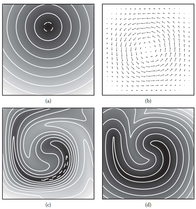
Velocity Field with Distortion

Eulerian advection schemes:

1. Begin with the field sampled on a grid

2. Reconstruct the field as a continuous function from the grid samples

3. Advect the reconstructed field

4. Resample the advected field on the grid

Though incompressible velocity field preserves volumes, at any point in space, the advected field may be stretched out along some axes and squished together along others.

For rendering, there is a local magnification (stretching out) along some axes and a local minification (squishing together) along the others.

Resampling a magnified field: doesnt’t lose information

Resampling a minified field: lose information, cause alias

Still from view of signal processing technology, minified field increase the frequency of singal.

Velocity Field without Distortion

Even for a pure translation velocity field with no distortion, the Nyquist limit essentially means that, the maximum spatial frequency that can be reliably advected has period .

The book says ? Does it should be ?

Higher-frequency signals, even though you might resolve them on the grid at a particular instant in time, cannot be handled in general: e.g., just in one dimension the highest-frequency component you can see on the grid, , exactly disappears from the grid once you advect it by a distance of .

Why highest-frequency component of 1D is ? Why it disappears by a distance of ?

Eulerian scheme filtering ability

A “perfect” Eulerian scheme would filter out the high-frequency components that can’t be reliably resampled at each time step, even as a bad one will allow them to alias as artifacts. The distortions inherent in non-rigid velocity fields mean that as time progresses, some of the lower-frequency components get transferred to higher frequencies—and thus must be destroyed by a good scheme. But note that the fluid flow, after squeezing the field along some axes at some point, may later stretch it back out—transferring higher frequencies down to lower frequencies. However, it’s too late if the Eulerian scheme has already filtered them out.

Is that what the author wants to express?

Becuase in non-rigid velocity fields, some of the lower-frequency components get transferred to higher frequencies.

So researcher that focus on fluid simulation precision should design a eulerian scheme that filter out the high-frequency components.

But for computer graphics, we need to keep high-frequency components as much as possible.

So that is why we turn to particles method?

Why DNS works well

At small enough length scales, viscosity and other molecular diffusion processes end up dominating advection. That means, : if is small enough, Eulerian schemes can behave perfectly well since the physics itself is effectively bandlimiting everything, dissipating information at higher frequencies.

That is why DNS works well.

But it is expensive for compute graphics.

Adaptive Grids

We have known that if is smaller, the Eulerian scheme will filter higher frequencies and keep higher bandwidth of low frequencies.

So adaptive grids can be used, where the grid resolution is increased wherever higher resampling density is required to avoid information loss, and decreased where the field is smooth enough that low resolution suffices.

Data Structure:

• Octrees

• Unstructured tetrahedral meshes

Complex, not really a solution to unwanted grid-caused diffusion

Store information in Particle

Store a field on particles that move with the flow

Then there is no filtering and no information loss

Particle methods apply best to fields with essentially zero diffusion (or viscosity, or conduction, or whatever other name is appropriate for the quantity in question).

Particle Advection

Error in particle advection: accumulated over many time steps

Error in the semi-Lagrangian method: being reset each time step

second-order Runge-Kutta

three-stage third-order Runge-Kutta scheme

Transferring Particles to the Grid

Common:

Particles track secondary field such as smoke concentration, foam, bubbles, or other things that would show up in rendering

Primary fluid variables like velocity store in grids.

But in PIC it is not…?

I come up with store velocity on particles firstly but not secondary field.

Maybe it is a differences in thinking between me and author.

I think when author says “track secondary field” first, he put PIC section to the next. It explains why author doesn’t say particles track velocity firstly.

Use kernel function to transfer value from particles to the grid.

Like SPH?

Particle Seeding

Make sure it’s consistent across different time steps and grid sizes.

My understanding is seeding should be related with delta time and grid size.

Diffusion

Particle-in-Cell Methods

Pressure projection to keep the velocity field divergence-free globally couples all the velocities together.

From Grid to Particle

For 2D, bilinear interpolation

For 3D, trilinear interpolation

Caution: For 2D as an example, if one grid velocity is undefined (the cell is not fluid), then in your bilinear interpolation, you only average three points. In other word, if is undefined, then right calcuation is but not .

Because undefined is not 0.

If you are using MAC grid, then grid position is not integer, it has an offset about h/2 from integer.

From Particles to Grid

Many particles may contributes the same one grid velocity,

but we are iterating all particles, so we should accumulate q and weight during the loop,

and calculate result in the last.

clear q and r for all cells

for all particles:
    q1 = q1 + w1 * qp
    q2 = q2 + w2 * qp
    q3 = q3 + w3 * qp
    q4 = q4 + w4 * qp

    r1 = r1 + w1
    r2 = r2 + w2
    r3 = r3 + w3
    r4 = r4 + w4

for all cells:
    q = q / r

PIC

PIC:

1. Velocity from particles to grids

2. Solve Advection in Grid

3. Interpolate back from grid to particles

4. Advect particles by the interpolated grid velocity field

About particles seeding: If too few particles in grid, seeding; if too many particles, delete the excess.

PIC suffers from severe numerial dissipation, because there is too many interpolation.

FLIP

In FLIP, instead of interpolating a quantity back to the particles, the change in the quantity (as computed on the grid) is interpolated.

So the delta quantity is used to increment the value in particles.

Each increment is smoothed because of interpolation, of course, but that is all. Smoothing is not accumulated, and thus FLIP is virtually free of numerical diffusion.

1. Velocity from particles to grids

   It stores a set of quantity

2. Solve Advection in Grid

   It stores a set of updated quantity

3. Get delta quantity in Grid

4. Interpolate back from grid to particles

5. Advect particles by the interpolated grid velocity field

PIC/FLIP

Eight particles pre grid cell, meaning there are more degrees of freedom in particles than in grid.

So FLIP may develop noise because the delta quantity is not enough to represent all degrees of motion.

Noise means velocity fluctuations on the particles may, on some time steps, average down to zero and vanish from the grid, and on other time steps show up as unexpected perturbations

But PIC doesn’t have the problem, because quantity is interpolated.

So a blending is useful, such as 0.01 PIC and 0.99 FLIP

Chapter 8: Water

Marker Particles and Voxels

Determining a cell is fluid or empty when water moves in or out of it. is the tricky part.

So one possibility is to define an initial level set of water, then advect is using sharp cubic interpolant.

But it still have problem about thin structures that thinner than about two grid cells. Droplets rarely can travel more than a few grid cells before disappearing.

This is where we turn instead to marker particles.

Marker Particles:

1. Emitting water particles to fill the volume of water

   If simulation has source, emit from it over time

2. Advect the particles

3. Mark the water cell: containing a marker particles is water, and the rest is empty or default

Density of marker particles

double of resolution: 4 particles in 2D, 8 in 3D

more may not bring improvement: sampling frequency is limited by grid resolution

So emitting particles in a random jittered pattern is a good idea. It is still considering about shearing flow that compresses along one axis and stretches along another can turn a regular lattice into weird anisotropic stripe-like patterns, far from a good uniform sampling.

Rendering

Need a smooth surface, we only have cells containing marker particles.

Blobbies

J. Blinn. A generalization of algebraic surface drawing. ACM Trans. Graph., 1(3):235–256, 1982

The blobby surface is implicitly defined as the points where

The blobby surface looks blobby. If using smoothing to mask blobby artifacts, the smoothing will also mask small-scale features.

An improvement on blobbies is given by Zhu and Bridson

One exciting direction is to skip the level set construction and directly use a triangle mesh to track the surface of the water.

1. Mesh may deform significantly, so remeshing is necessary.

2. Mesh spiltting and merging need topology change operation.

3. Numerical errors can cause the mesh to collide with itself.

Combine marker particles and FLIP

If we have already use particles, why not get th full benefit from them?

So using FLIP instead of semi-Lagrangian method.

Here you will realize that FLIP is not a solver, it is just a advection method comparing with semi-Largrangian method.

Combination:

1. From the particles, construct the level set for the liquid.

2. Transfer velocity (and any other additional state) from particles to the grid, and extrapolate from known grid values to at least one grid cell around the fluid, giving a preliminary velocity field

3. Add body forces such as gravity or artistic controls to the velocity field.

4. Construct solid level sets and solid velocity fields.

5. Solve for and apply pressure to get a divergence-free velocity that respects the solid boundaries.

6. Update particle velocities by interpolating the grid update to add to the existing particle velocities (FLIP), or simply interpolating the grid velocity (PIC), or a mix thereof.

7. Advect the particles through the divergence-free velocity field

The final step should be advecting the particels through particles velocity? Instead of divergence-free velocity in grid? Or the “divergence-free velocity ” means velocity in particles?

Why we need More Accurate Pressure Solves: Voxelized Surface

Marker particles method create block voxelized surface in field value.

Simulation core is pressure solving

Pressure solving only see a block voxelized surface, so as a solving result, velocity filed cannot avoid significant voxel artifacts.

For example, small “ripples” less than a grid cell high do not show up at all in the pressure solve, and thus they aren’t evolved correctly but rather persist statically in the form of a strange displacement texture.

So we need to inform the pressure solver about the location of the water-air interface. Then we modify the pressure solver, about how we compute the gradient of pressure near the water-air interface for updating velocities. It naturally will also changes the matrix in the pressure equations.

We modify pressure solver and add an additional process about water-air interface?

OK. See the ghost fluid method section, I realize it is about how to determine location.

Ghost fluid Method

Assume that we have known that how to update velocity:

Suppose that is in the water, i.e. and is in the air, i.e. .

Simple solver, which causes voxelized surface, set .

But it would be more accurate to say that happens at the water-air interface, and doesn’t represent interface.

So we set a to present the “ghost” pressure in the air. Now the update is:

Now we should solve the unknown , we know we should use the water-air interface condition that:

Where means we do linearly interpolating between and gives the location of the interface at where

Solve :

and then substitute it into update eq:

that is all.

Fig: Ghost fluid Method

Other methods …

Topology Change and Wall Separation

How does Separation happen

Why water will separation?

Only considering numerical scheme, if water is path-connected, then after advection, it must remain path-connected. In other word, in theory, if velocity field path-connected, then it will never separate.

But in real simulation, if you use level set or marker particles method, you will find the separation happens natually. But it may just caused by numerical error.

Lose volume when merging water

A water drop can penetrate quite deeply into a solid wall or into another water region during advection, effectively losing volume in the process.

How Liquid can Separate from Solid Walls

In fact, exactly what happens at the moving contact line where air, water, and solid meet is again not fully understood. Complicated physical chemistry, including the influence of past wetting (leaving a nearly invisible film of water on a solid), is at play.

Other searcher …

Volume Control

Because of pressure solving error, truncation error in level set representation, advection error, as well as the topology issues noted above, it is not surprising that fluid volume can’t be conserve.

Other searcher …

Surface Tension

Both graphics and scientific computing, are studying how to add surface tension.

Other searcher …